Time Window
When using the Time Window Aggregation template to develop stream processing jobs, you need to configure the window strategy. Some of the key concepts for time window are introduced below.
Event time
Data aggregation is usually based on the event time, which is the time when the event occurs. Every event has a corresponding timestamp, which is part of the data record. This timestamp is the event time. When the event time is used to define a time window, the stream processing engine can process disordered event streams and event time deviations, and compute meaningful results based on the time when the event actually occured.
Time window
The EnOS Stream Processing Engine is based on time windows (micro-batch model) and processes data at the specified window size (interval of batch size). Windowing is simply the notion of taking a data source and chopping it up along temporal boundaries into finite chunks for processing, which determines how often a stream computing task gets the data. The EnOS Streaming Processing Engine supports tumbling window operations.
The division of time window starts at 00:00:00 on January 1, 1970 GMT. When data in a time window arrives (based on the event time), the time window is generated.
Tumbling window
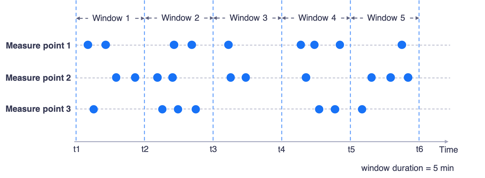
Tumbling windows have a fixed size and do not overlap. Data belonging to a window will be aggregated with the specified method. In the figure below for example, the tumbling window has a size of 5 minutes. Each window starts and is evaluated every 5 minutes without any overlapping, with each representing a specific time segment.

Window latency
Generally, when a window closes, the data processing in the window should have been completed, and a new window will start. However, data transfer might be delayed because of various factors like device failure and transmission efficiency. This is where window latency comes in.
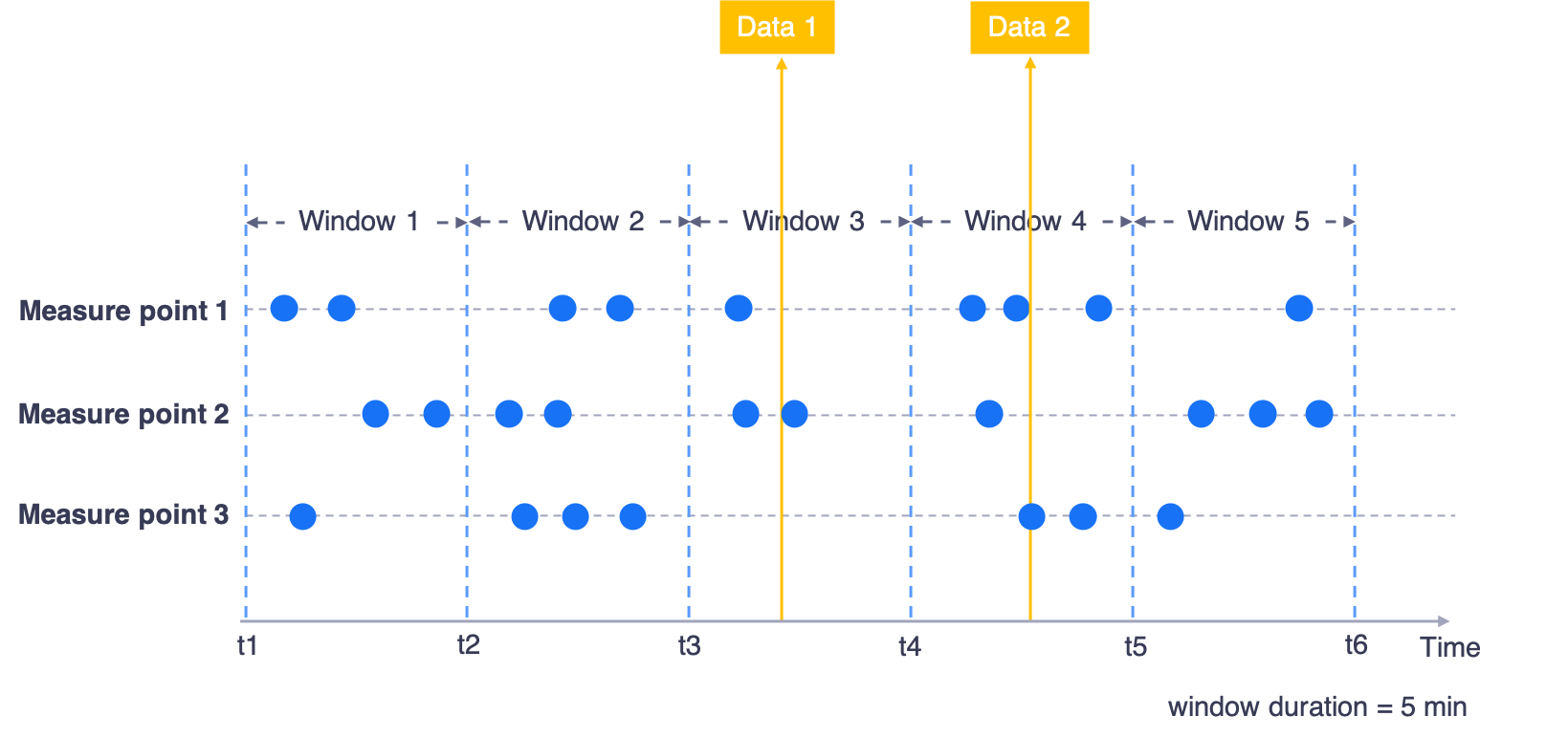
Latency setting is introduced to extend the validity time of the window after it closes. Late data arriving within the specified extension period will be added to the window and computed again and those that arrive after will be ignored.
In the following example, the window size is 5 minutes, and Data 1 and Data 2 are late/delayed data. Window 2 contains data that falls in the time range between 11:00 and 11:05. If latency is not enabled, Window 2 will be closed at 11:05, and Data 1 and Data 2 will be ignored. If a latency of 5 minutes is enabled, Data1 will be added to Window 2 for computing again, and Data 2 will be ignored.
